In my previous
article, I introduced you to the basics of Apache Spark, different data representations (RDD / DataFrame / Dataset) and basics of operations (Transformation and Action). We even solved a machine learning problem from one of our past
hackathons. In this article, I will continue from the place I left in my previous article. I will focus on manipulating RDD in PySpark by applying operations (Transformation and Actions).
As you would remember, a RDD (Resilient Distributed Database) is a collection of elements, that can be divided across multiple nodes in a cluster to run parallel processing. It is also a fault tolerant collection of elements, which means it can automatically recover from failures. RDD is immutable, i.e. once created, we can not change a RDD. So, then how do I apply operations on a RDD? Well, we apply an operation and store results in another RDD
For this article, one must have some understanding about Apache Spark and hands on experience in python programming.
Table of Contents
- Recap
- What is Transformation and Action?
- Transformation and Action
- Major Categories
- Applying Transformation and Action
- General
- Mathematical and Statistical
- Set Theory and Relational
- Data-structure and IO
Recap
Let’s recall concepts about RDD from our
previous article:
- We can create a RDD in two different ways, from existing source and external source.
- We can apply two types of operations on RDD, namely “transformation” and “action”. All transformations on RDD are lazy in nature, which means that computations on RDD are not done until we apply an action.
- RDDs are immutable in nature i.e. we cannot change the RDD, we need to transform it by applying transformation(s). There are various transformations and actions, which can be applied on RDD.
Before applying transformations and actions on RDD, we need to first open the PySpark shell (please refer to my previous
article to setup PySpark ).
$ ./bin/pyspark
What is Transformation and Action?
Spark has certain operations which can be performed on RDD. An operation is a method, which can be applied on a RDD to accomplish certain task. RDD supports two types of operations, which are Action and Transformation. An operation can be something as simple as sorting, filtering and summarizing data.
Let’s take few examples to understand the concept of transformation and action better. Let’s assume, we want to develop a machine learning model on a data set. Before applying a machine learning model, we will need to perform certain tasks:
- Understand the data ( List out the number of columns in data and their type)
- Preprocess the data (Remove null value observations on data).
- Filter the data (Let’s say, we want to filter the observations corresponding to males data)
- Fill the null values in data ( Filling the null values in data by constant, mean, median, etc)
- Calculate the features in data
All the above mentioned tasks are examples of an operation. In Spark, operations are divided into 2 parts – one is transformation and second is action. Find below a brief descriptions of these operations.
Transformation: Transformation refers to the operation applied on a RDD to create new RDD. Filter, groupBy and map are the examples of transformations.
Actions: Actions refer to an operation which also applies on RDD, that instructs Spark to perform computation and send the result back to driver. This is an example of action.
The Transformations and Actions in Apache Spark are divided into 4 major categories:
- General
- Mathematical and Statistical
- Set Theory and Relational
- Data-structure and IO
Applying Transformation and Action
To understand the operations, I am going to use the text file from my previous article. Let’s begin, I have already copied and pasted all text from my blog in a textfile called blogtexts. To download this file you can refer to this
link. Before applying operations on blogtexts, we need to first load this file with the help of SparkContext.
rdd = sc.textFile("PATH/blogtexts")
In above code, ‘PATH’ is the location of blogtexts. Let’s see first 5 elements of RDD.
rdd.take(5)
Output:
[u'Think of it for a moment \u2013 1 Qunitillion = 1 Million Billion! Can you imagine how many drives / CDs / Blue-ray DVDs would be required to store them? It is difficult to imagine this scale of data generation even as a data science professional. While this pace of data generation is very exciting,  it has created entirely new set of challenges and has forced us to find new ways to handle Big Huge data effectively.',
 u'',
 u'Big Data is not a new phenomena. It has been around for a while now. However, it has become really important with this pace of data generation. In past, several systems were developed for processing big data. Most of them were based on MapReduce framework. These frameworks typically rely on use of hard disk for saving and retrieving the results. However, this turns out to be very costly in terms of time and speed.',
 u'',
 u'On the other hand, Organizations have never been more hungrier to add a competitive differentiation through understanding this data and offering its customer a much better experience. Imagine how valuable would be Facebook, if it did not understand your interests well? The traditional hard disk based MapReduce kind of frameworks do not help much to address this challenge.'
]
Now lets see one by one how transformations and actions work on RDDs.
General transformations
For each transformation, I have first laid out the need of the transformation in the form of a question and then answered it in the subsequent section.
Transformation: map and flatMap
Q1: Convert all words in a rdd to lowercase and split the lines of a document using space.
To lower the case of each word of a document, we can use the map transformation. A map transformation is useful when we need to transform a RDD by applying a function to each element. So how can we use map transformation on ‘rdd’ in our case?
Solution: Let’s see through the example, Apply a function called “Func” on each words of a document ( blogtexts ). “Func” will do two things:
- It will take a corpus, lower the each words in this corpus.
- After that it splits the words in each line by space.
To do this first we need to write “Func” and then apply this function using map.
def Func(lines):
      lines = lines.lower()
      lines = lines.split()
      return lines
rdd1 = rdd.map(Func)
After applying the function (Func) on “rdd”, we have transformed this “rdd” into “rdd1”, we can see the first 5 elements of “rdd1” by applying take operation (which is an action).
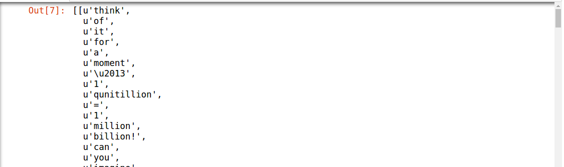
rdd1.take(5)
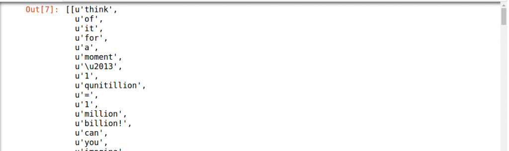
Output is too long so, I have just attached a snippet of it. We can also see that our output is not flat (it’s a nested list). So for getting the flat output, we need to apply a transformation which will flatten the output, The transformation “flatMap” will help here:
The “flatMap” transformation will return a new RDD by first applying a function to all elements of this RDD, and then flattening the results. This is the main difference between the “flatMap” and map transformations. Let’s apply a “flatMap” transformation on “rdd” , then take the result of this transformation in “rdd2” and print the result after applying this transformation.
rdd2 = rdd.flatMap(Func)
rdd2.take(5)
Output: [u'think', u'of', u'it', u'for', u'a']
You can now observe that the new output is flattened out.
Transformation: filter
Q2: Next, I want to remove the words, which are not necessary to analyze this text. We call these words as “stop words”; Stop words do not add much value in a text. For example, “is”, “am”, “are” and “the” are few examples of stop words.
Solution: To remove the stop words, we can use a “filter” transformation which will return a new RDD containing only the elements that satisfy given condition(s). Lets apply “filter” transformation on “rdd2” and get words which are not stop words and get the result in “rdd3”. To do that:
- We need to define the list of stop words in a variable called “stopwords” ( Here, I am selecting only a few words in stop words list instead of all the words).
- Apply “filter” on “rdd2” (Check if individual words of “rdd2” are in the “stopwords” list or not ).
We can check first 10 elements of “rdd3” by applying take action.
stopwords = ['is','am','are','the','for','a']
rdd3 = rdd2.filter(lambda x: x not in stopwords)
rdd3.take(10)
Output:
[u'think',
 u'of',
 u'it',
 u'moment',
 u'\u2013',
 u'1',
 u'qunitillion',
 u'=',
 u'1',
 u'million']
After seeing the result of a filter transformation, we can check now we don’t have specified stop words in rdd3 (there are no for and a).
Transformation: groupBy
Q3: After getting the results into rdd3, we want to group the words in rdd3 based on which letters they start with. For example, suppose I want to group each word of rdd3 based on first 3 characters.
Solution: The “groupBy” transformation will group the data in the original RDD. It creates a set of key value pairs, where the key is output of a user function, and the value is all items for which the function yields this key.
- We have to pass a function (in this case, I am using a lambda function) inside the “groupBy” which will take the first 3 characters of each word in “rdd3”.
- The key is the first 3 characters and value is all the words which start with these 3 characters.
After applying “groupBy” function, we store the transformed result in “rdd4” (RDDs are immutable – remember!). To view “rdd4”, we can print first (key, value) elements in “rdd4”.
rdd4 = rdd3.groupBy(lambda w: w[0:3])
print [(k, list(v)) for (k, v) in rdd4.take(1)]
Output: [(u'all', [u'all', u'allocates', u'all', u'all', u'allows', u'all', u'all', u'all', u'all', u'all', u'all', u'all'])]
Transformation: groupByKey / reduceByKey
Q4: What if we want to calculate how many times each word is coming in corpus ?
Solution: We can apply the “groupByKey” / “reduceByKey” transformations on (key,val) pair RDD. The “groupByKey” will group the values for each key in the original RDD. It will create a new pair, where the original key corresponds to this collected group of values.
To use “groupbyKey” / “reduceByKey” transformation to find the frequencies of each words, you can follow the steps below:
- A (key,val) pair RDD is required; In this (key,val) pair RDD, key is the word and val is 1 for each word in RDD (1 represents the number for the each word in “rdd3”).
- To apply “groupbyKey” / “reduceByKey” on “rdd3”, we need to first convert “rdd3” to (key,val) pair RDD.
Let’s see, how to convert “rdd3” to new mapped (key,val) RDD. And then we can apply “groupbyKey” / “reduceByKey” transformation on this RDD.
rdd3_mapped = rdd3.map(lambda x: (x,1))
rdd3_grouped = rdd3_mapped.groupByKey()
In the above code I am first converting “rdd3” into “rdd3_mapped”. The “rdd3_mapped” is nothing but a mapped (key,val) pair RDD. Then I am applying “groupByKey” transformation on “rdd3_mapped” to group the all elements based on the keys (words). Next, I am saving the result into “rdd3_grouped”. Let’s see the first 5 elements in “rdd3_grouped”.
print(list((j[0], list(j[1])) for j in rdd3_grouped.take(5)))
Output: [(u'all', [1, 1, 1, 1, 1, 1, 1, 1, 1, 1]), (u'elements,', [1, 1]), (u'step2:', [1]), (u'manager', [1]), (u'(if', [1])]
After seeing the result of the above code, I rechecked the corpus to know, how many times the word ‘manager’ is there, so I found that ‘manager’ is written more then once. I figure out that there are more words like ‘manager.’ , ‘manager,’ and ”manager:’. Let’s filter ‘manager,’ in “rdd3”.
rdd3.filter(lambda x: x == 'manager,').collect()
Output: [u'manager,', u'manager,', u'manager,']
We can see that in above output, we have multiple words with ‘manager’ in our corpus. To overcome this situation we can do several things. We could apply a regular expression to remove unnecessary punctuation from the words. For the purpose of this article, I am skipping that part.
Until now we have not calculated the frequencies / counts of each words. Let’s proceed further :
rdd3_freq_of_words = rdd3_grouped.mapValues(sum).map(lambda x: (x[1],x[0])).sortByKey(False)
In the above code, I first applied “mapValues” transformation on “rdd3_grouped”. The “mapValues” (only applicable on pair RDD) transformation is like a map (can be applied on any RDD) transform but it has one difference that when we apply map transform on pair RDD we can access the key and value both of this RDD but in case of “mapValues” transformation, it will transform the values by applying some function and key will not be affected. So for example, in above code I applied sum, which will calculate the sum (counts) for the each word.
After applying “mapValues” transformation I want to sort the words based on their frequencies so for doing that I am first converting a ( word, frequency ) pair to ( frequency,word ) so that our key and values will be interchanged then, I will apply a sorting based on key and then get a result in “rdd3_freq_of_words”. We can see that 10 most frequent words I used in my previous blog by applying “take” action.
rdd3_freq_of_words.take(10)
output:
[(164, u'to'),
 (143, u'in'),
 (122, u'of'),
 (106, u'and'),
 (103, u'we'),
 (69, u'spark'),
 (64, u'this'),
 (63, u'data'),
 (55, u'can'),
 (52, u'apache')]
Above output shows that I used words spark 69 times and Apache 52 times in my previous blog.
We can also use “reduceByKey” transformation for counting the frequencies of each word in (key,value) pair RDD. Lets see how will we do this.
rdd3_mapped.reduceByKey(lambda x,y: x+y).map(lambda x:(x[1],x[0])).sortByKey(False).take(10)
output:
[(164, u'to'),
 (143, u'in'),
 (122, u'of'),
 (106, u'and'),
 (103, u'we'),
 (69, u'spark'),
 (64, u'this'),
 (63, u'data'),
 (55, u'can'),
 (52, u'apache')]
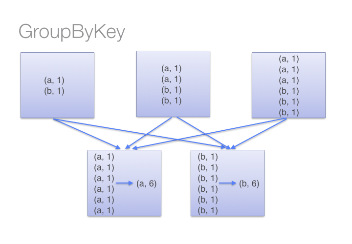
If we compare the result of both ( “groupByKey” and “reduceByKey”) transformations, we have got the same results. I am sure you must be wondering what is the difference in both transformations. The “reduceByKey”transformations first combined the values for each key in all partition, so each partition will have only one value for a key then after shuffling, in reduce phase executors will apply operation for example, in my case sum(lambda x: x+y).
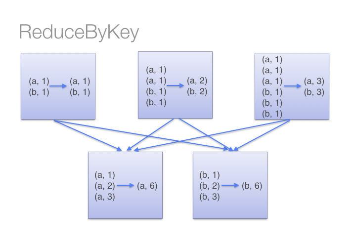
Source: Databricks
But in case of “groupByKey” transformation, it will not combine the values in each key in all partition it directly shuffle the data then merge the values for each key. Here in “groupByKey” transformation lot of shuffling in the data is required to get the answer, so it is better to use “reduceByKey” in case of large shuffling of data.
Source: Databricks
Transformation: mapPartitions
Q5: How do I perform a task (say count the words ‘spark’ and ‘apache’ in rdd3) separatly on each partition and get the output of the task performed in these partition ?
Soltion: We can do this by applying “mapPartitions” transformation. The “mapPartitions” is like a map transformation but runs separately on different partitions of a RDD. So, for counting the frequencies of words ‘spark’ and ‘apache’ in each partition of RDD, you can follow the steps:
- Create a function called “func” which will count the frequencies for these words
- Then, pass the function defined in step1 to the “mapPartitions” transformation.
def func(iterator):
  count_spark = 0
  count_apache = 0
  for i in iterator:
     if i =='spark':
        count_spark = count_spark + 1
     if i == 'apache':
        count_apache = count_apache + 1
  return (count_spark,count_apache)
Lets apply above function called ‘func’ on each partition of rdd3.
rdd3.mapPartitions(func).glom().collect()
Output: [[49, 39], [20, 13]]
I have used the “glom” function which is very useful when we want to see the data insights for each partition of a RDD. So above result shows that 49,39 are the counts of ‘spark’, ‘apache’ in partition1 and 20,13 are the counts of ‘spark’, ‘apache’ in partition2. If we won’t use the “glom” function we won’t we able to see the results of each partition.
rdd3.mapPartitions(f).collect()
Output: [49, 39, 20, 13]
Math / Statistical Transformation
Transformation: sample
Q6: What if I want to work with samples instead of full data ?
Soltion: “sample” transformation helps us in taking samples instead of working on full data. The sample method will return a new RDD, containing a statistical sample of the original RDD.
We can pass the arguments insights as the sample operation:
- “withReplacement = True” or False (to choose the sample with or without replacement)
- “fraction = x” ( x= .4 means we want to choose 40% of data in “rdd” ) and “seed” for reproduce the results.
rdd3_sampled = rdd3.sample(False, 0.4, 42)
print len(rdd3.collect()),len(rdd3_sampled.collect())
Output: 4768 1895
We can see the above output, we have total 4768,1895 words in “rdd3” and “rdd3_sampled”.
Set Theory / Relational Transformation
Transformation: union
Q 7: What if I want to create a RDD which contains all the elements (a.k.a. union) of two RDDs ?
Solution: To do so, we can use “union” transformation on two RDDs. In Spark “union” transformation will return a new RDD by taking the union of two RDDs. Please note that duplicate items will not be removed in the new RDD. To illustrate this:
- I am first going to create a two sample RDD ( say sample1, sample2 ) from the “rdd3” by taking 20% sample for each.
- Apply a union transformation on sample1, sample2.
sample1 = rdd3.sample(False,0.2,42)
sample2 =rdd3.sample(False,0.2,42)
union_of_sample1_sample2 = sample1.union(sample2)
print len(sample1.collect()), len(sample2.collect()),len(union_of_sample1_sample2.collect())
Output: 914 914 1828
From the above output, we can see that the “sample1”, “sample2” both have 914 elements each. And in the “union_of_sample1_sample2”, we have 1828 elements which shows that union operation didn’t remove the duplicate elements.
Transformation: join
Q 8: If we want to join the two pair RDDs based on their key.
Solution: The “join” transformation can help us join two pairs of RDDs based on their key. To show that:
- First create the two sample (key,value) pair RDDs (“sample1”, “sample2”) from the “rdd3_mapped” same as I did for “union” transformation
- Apply a “join” transformation on “sample1”, “sample2”.
sample1 = rdd3_mapped.sample(False,.2,42)
sample2 = rdd3_mapped.sample(False,.2,42)
join_on_sample1_sample2 = sample1.join(sample2)
join_on_sample1_sample2.take(2)
Output: [(u'operations', (1, 1)), (u'operations', (1, 1))]
Transformation: distinct
Q 9: How to calculate distinct elements in a RDD ?
Solution: We can apply “distinct” transformation on RDD to get the distinct elements. Let’s see how many distinct words do we have in the “rdd3”.
rdd3_distinct = rdd3.distinct()
len(rdd3_distinct.collect())
Output: 1485
“rdd3_distinct” will contain all the unique words / elements present in “rdd3”. We can also check that we have 1485 unique words in the “rdd3”.
Data Structure / I/O Transformation
Transformation: coalesce
Q 10: What if I want to reduce the number of partition of a RDD and get the result in a new RDD?
Solution: We will use “coalesce” transformation here. To demonstrate that:
- Let’s first check the number of partition in rdd3.
rdd3.getNumPartitions()
Output: 2
2. And now apply coalesce transformation on “rdd3” , get the results in “rdd3_coalesce” and see the number of partitions.
rdd3_coalesce = rdd3.coalesce(1)
rdd3_coalesce.getNumPartitions()
Output: 1
In some previous examples of transformation I already used some of the actions on different RDDs for printing the result. For example,”take” to print the first n elements of a RDD , “getNumPartitions” to know how many partition a RDD has and “collect” to print all elements of RDD.
Now, I will take few more actions to demonstrate how we can get the results.
General Actions
Action: getNumPartitions
Q 11: How do I find out number of parition in RDD ?
Solution: With “getNumPartitions”, we can find out that how many partitions exist in our RDD. Let’s see how many partition our initial RDD ("rdd3") has.
rdd3.getNumPartitions() Output: 2
Action: Reduce
Q 12: If I want to find out the sum the all numbers in a RDD.
Solution: To demonstrate this, I will:
- First create a RDD from a list of number from (1,1000) called “num_rdd”.
- Use a reduce action and pass a function through it (lambda x,y: x+y).
A reduce action is use for aggregating all the elements of RDD by applying pairwise user function.
num_rdd = sc.parallelize(range(1,1000))
num_rdd.reduce(lambda x,y: x+y)
Output: 499500
In the code above, I first created a RDD(“num_rdd”) from the list and then I applied a reduce action on it to sum all the numbers in “num_rdd”.
Mathematical / Statistical Actions
Action: count
Q 13: Count the number of elements in RDD.
Solution: The count action will count the number of elements in RDD. To see that, let’s apply count action on “rdd3” to count the number of words in "rdd3".
rdd3.count() Output: 4768
Action: max, min, sum, variance and stdev
To take the maximum, minimum, sum, variance and standard deviation of a RDD, we can apply “max”, “min”, “sum”, “variance” and “stdev” actions. Let’s take the maximum, minimum, sum, variance and standard deviation of “num_rdd”.
num_rdd.max(),num_rdd.min(), num_rdd.sum(),num_rdd.variance(),num_rdd.stdev()
Output: (999, 1, 499500, 83166.66666666667, 288.38631497813253)
End Note
Taking a step back, we got introduced to the fascinating world of Apache Spark in the last article. In this article, I have introduced you to some of the most common transformations and actions on RDD. There are many more transformations and actions defined on RDDs, but it is cumbersome (and unwanted) to cover all of them in one article. To learn more about transformations and actions, you can refer RDD API
doc in Python.
I suggest you to apply these operations at your end in RDD, and get hands on experience on what are the challenges you are face while applying these. Let me know your doubts & any challenges you face in the comments section and I would be happy to answer them.
Also, if you have any questions or suggestions about other features of RDD that you would like to know about, please drop in your comments below. In the next article, I’ll discuss about Dataframe operations in PySpark.
You can test your skills and knowledge. Check out Live Competitions and compete with best Data Scientists from all over the world.